Semi-Supervised Learning and MixMatch
이 글에서는 Semi-Supervised Learning이란 무엇이고, 이와 관련한 연구 중 하나인 MixMatch 논문과 후속 연구들에 대해 소개하고자 합니다.
먼저 Semi-Supervised Learning에 대해 소개하고, 그 다음 논문 리스트이자, 이 글의 순서는 다음과 같습니다.
- MixMatch: A Holistic Approach to Semi-Supervised Learning
- ReMixMatch: Semi-Supervised Learning with Distribution Alignment and Augmentation Anchoring
- FixMatch: Simplifying Semi-Supervised Learning with Consistency and Confidence
Semi-Supervised Learning
What is Semi-Supervised Learning?
먼저, Semi-Supervised Learning(SSL)은 그야말로, Supervised Learning과 Unsupervised Learning을 섞은 형태입니다. 즉, labeled data와 unlabeled data를 적절하게 합쳐서 학습을 하게 됩니다.
Why Semi-Supervised Learning?
사실, Semi-Supervised Learning은 Supervised Learning의 성능을 넘어설 수 없습니다. 그럼, 왜 Semi-Supervised Learning이 필요할까요? 우리는 현실적으로 모든 데이터에 레이블, 즉 \(y\)를 가진 데이터를 찾기가 어렵습니다.
하지만 앞서 말씀드렸듯 우리는 성능이 더 좋은 Supervised Learning을 활용하고 싶습니다. 따라서 label이 없다면? 만들면 됩니다! 하고 data labeling을 시도할 수 있습니다. 하지만 labeling은 많은 시간과 비용이 듭니다. 예를 들어, 의료 이미지 데이터를 학습시키고 싶은데, labeling이 필요하다면 값비싼 전문가들에게 요청을 해야할 것입니다. 따라서 우리는, 레이블 데이터를 가지기도, 추가로 얻기도 꽤나 어려운 상황입니다.
그럼에도 불구하고 우리는 최대한 좋은 성능을 낼 수 있는 머신러닝을 적용해야 하기 때문에, Unsupervised 형태가 아닌 조금이라도 가지고 있는 labeled data를 활용하는 Semi-Supervised Learning을 고려하게 됩니다.
Yes, Semi-Supervised Learning!
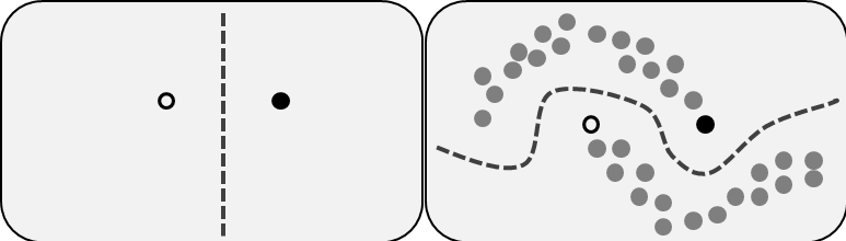 Semi-Supervised Learning: source: Wikipedia
위의 그림은 Semi-Supervised Learning을 잘 설명해주는 그림입니다. 먼저 왼쪽 그림을 보면, 우리는 labeled data points를 2개 가지고 있다고 생각해봅시다. 실제로 supervised learning으로 classfication을 위한 decision boundary를 만들 때 위와 같이 만들(예를 들어, 두 data의 margin을 최대화하는 식으로) 수 있습니다. 하지만, 우리는 실제로 수많은 unlabeled data가 있고, 오른쪽 그림에서 볼 수 있듯이 왼쪽의 decision boundary로는 택도 없는 다른 분류를 하게 됩니다.
따라서, Semi-Supervised Learning으로 unlabeled data를 함께 고려하여 data의 distribution을 더 잘 추정하려 하고, 그로부터 classification, regression 등의 supervised learning task를 잘 풀 수 있게 됩니다.
그렇다면, Semi-Supervised Learning을 통해 data distribution을 더 잘 추정할 수 있고 실제로 unseen data가 주어졌을 때 더 generalization을 잘 하게 됩니다. 또한, supervised learning과 비교해서 더 적은 labeled data로 충분히 비슷한 성능을 낼 수 있도록 잘 학습하는 것이 목표이자 장점입니다.
이 글에선 Semi-Supervised Learning 중의 하나인 MixMatch에 관해 설명하겠습니다. 이 논문은 NeurIPS 2019에서 Google Research가 낸 논문입니다. 그리고, MixMatch의 후속 연구들인 ReMixMatch, FixMatch에 대해 설명하고자 합니다.
MixMatch: A Holistic Approach to Semi-Supervised Learning
MixMatch는 아래의 3가지 SSL의 Related Work를 합친 방법입니다. 이에 대해 소개하고자 합니다.
1. Related Work
1-1. Consistency Regularization
Consistency는, 우리가 input data를 augmentation한 것에 대한 prediction의 일관성을 의미합니다.
예를 들어, 우리가 이미지 데이터를 가지고 있다고 합시다. 아래 이미지의 맨 왼쪽 그림입니다. 이 이미지를 회전하고, 끝을 자르고, 대칭 변환으로 하여 변형시키는 방법입니다.
 Data Augmentation: source: http://www.aitimes.com/news/articleView.html?idxno=132226
원래 이미지가 사람이라면, 사람이 이미지 안에 있다는 하에 회전하고 끝 부분을 자르고, 좌우 대칭을 시켜도 사람임은 같을 것입니다. 즉, 모델에서 이 augmented된 데이터를 넣어서 학습을 시켜도 예측값은 같아야 잘 학습된 것일 겁니다.
그렇다면, Consistency가 의미하는 바는, 약간 변형한 데이터를 넣어도 “일관되게” 같은 예측을 출력할 수 있도록 하는 것입니다.
자, 이게 왜 중요할까요? 우리는 Semi-Supervised Learning에서 labeled와 unlabeled data를 이용해 데이터를 학습할텐데, 비슷한 데이터 혹은 약간 변형한 데이터를 가지고 학습을 시켰을 때 예측이 비슷해야겠죠? 그걸 label이 없는 상황에서도 일관되게 학습을 잘 하도록 하는 것이 SSL의 과정입니다.
수식적으로는 다음과 같이 표현할 수 있습니다.
\[\| p(y|\mathrm{Augment}(x);\theta)-p(y|\mathrm{Augment}(x);\theta) \|_2^2\]논문에서는 예시로 L2 loss를 사용하였지만 사실 어떤 loss 든 정의하기 나름일겁니다. 수식에서 \(\textrm{Augment}(\cdot)\)은 stochastic data augmentation을 의미하므로 다른 값입니다. 수식을 통해 모델은 augmented된 data에 대해 같은 class로 분류하도록 학습됨을 알 수 있습니다. 그리고, unlabeled data라면, augmentation 후에도 같은 class를 갖도록, 같은 class로 분류될 확률이 크도록 학습이 되어야 할 것입니다.
1-2. Entropy Minimization
Entropy Minimization은 모델(Classifier)가 unlabeled data의 예측 entropy를 최소화하는 것입니다. 이는, unlabeled data에 대한 예측을 확신하도록, 해당 class에 대한 prediction probability를 높이도록 학습함을 의미합니다.
Entropy Minimization의 방법 중에는 Pseudo-Labeling이 있습니다. 이는 unlabeled data에 대해 confidence를 높여서 implicit하게 예측을 하고 이 예측한 label을 출력하는 것입니다. 이는 학습에 다시 포함될 수도 있습니다.
(그림을 넣어 설명해보자.)
1-3. MixUp
MixUp은 이 방법이 소개된 아래의 그림으로 설명하고자 합니다.
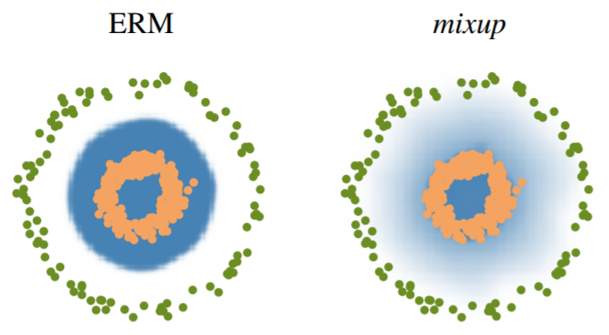 MixUp
MixUp
초록색을 Class 1, 주황색을 Class 2, 파란색은 prediction probability라고 합시다. 우리는 class1과 class2를 확실하게 알지만, 이에 대해 약간 섞어, class 1인 애들을 class 1일 확률이 0.8, 2일 확률이 0.2 정도로 섞습니다. 그럼, 데이터는 약간 변형되고 약간 이상하지만 충분히 우리가 모르는 데이터 내에 있을 수 있는 정도의 데이터로 모델은 학습하게 됩니다. 이것도 가짜 label이 형성되면서 이 perturbation에 대해 모델은 robust하게 학습이 될 수 있습니다!
2. MixMatch
앞에서 MixMatch는 위의 Related Work를 모두 합친 방법이라고 언급했습니다. 이를 염두하고 이제 MixMatch에 대해 소개하겠습니다.
2-1. Problem Setting
2-2. Overview
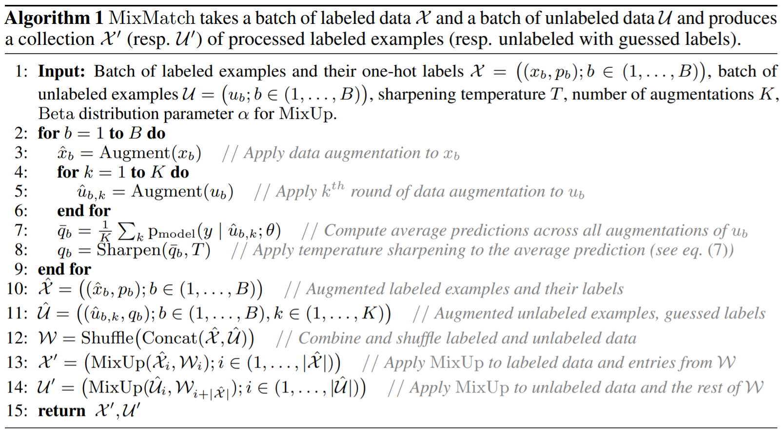
MixMatch의 알고리즘이자, 전체적인 Overview는 다음과 같이 요약할 수 있습니다.
MixMatch
Given \(\mathcal{X},\mathcal{U},T,K,\alpha\)
Data Augmentation to labeled data \(x\) and unlabeled data \(u\)
Compute average prediction of augmented unlabeled data \(\hat{u}_{b,k}\)
Compute sharpening function to average of guessed labels for temperature
Repeat 2-4. each iteration number, each batch
Return augmented labeled and unlabeled data
Learning and Prediction
- Get each batch of augmented labeled and unlabeled data from MixMatch
Loss function about labeled data and unlabeled data
\[\mathcal{L}_{\mathcal{X}}=\frac{1}{|\mathcal{X}'|}\sum_{x,p \in \mathcal{X}'}H(p,p_{\textrm{model}}(y|x;\theta)) \qquad (3) \\\] \[\mathcal{L}_{\mathcal{U}}=\frac{1}{L|\mathcal{U}'|}\sum_{u,q \in \mathcal{U}'}\|q-p_{\textrm{model}}(y|u;\theta)\|_2^2 \qquad(4)\]Total Loss function
\[\mathcal{L}=\mathcal{L}_{\mathcal{X}}+\lambda_{\mathcal{U}}\mathcal{L}_{\mathcal{U}} \qquad (5)\]
2-3. Method
이제, 각 과정을 설명하고자 합니다.
1. Data Augmentation
먼저, labeled data \(x_b \in \mathcal{X}\) 와 unlabeled data\(u_b \in \mathcal{U}\)를 augmentation합니다.
\(\hat{x}_b = \textrm{Augment}(x_b) \\ \hat{u}_{b,k} = \textrm{Augment}(u_b)\) 2. Label Guessing
위에서 augmented된 data를 이용해 분류, 예측합니다. 이렇게 예측한 클래스 레이블을 guessed label \(q_b\)라 합니다. 그리고, 이 예측한 클래스 확률을 평균을 냅니다. 이를 \(\bar{q}_b\)라 합니다.
\[\bar{q}_b=\frac{1}{K}\sum_{k=1}^K p_{\textrm{model}}(y|\hat{u}_{b,k};\theta)\]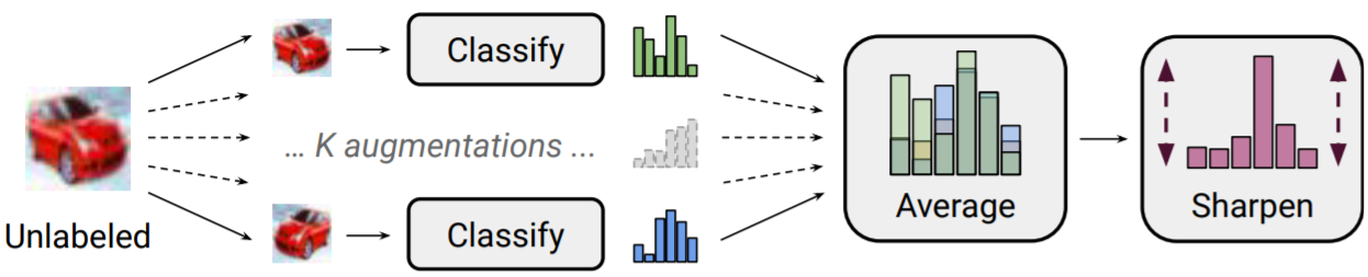 Label Guessing
3. Sharpening
이제 이에 대해 Entropy Minimization을 하기 위해 Sharpening합니다. 다시 말해, 우리가 augmentation된 unlabeled data로도 분류를 잘 하기 위해 하나의 예측된 클래스의 확률을 가장 높이고 나머지 다른 클래스에 대한 확률을 줄임으로써 예측에 대한 불확실성, 즉 entropy를 줄입니다. 이는 위의 그림에서 잘 나타나 있습니다.
자, 다시 말해, 아래의 sharpen function을 이용해 guessed label(의 평균)의 entropy(불확실성)을 최소화합니다. 아래 함수를 이용해 temper하게 하고 temperature를 낮추는 것은 모델이 entropy가 낮도록 예측하게 하는 것입니다.
\[\textrm{Sharpen}(\bar{q}_b,T)_i := \frac{\bar{q}_{b,i}^{\frac{1}{T}}}{\sum_{j=1}^L\bar{q}_{b,j}^{\frac{1}{T}}} \qquad(7)\]4. MixUp
이제, 위에서 augmented되고 entropy가 minimize된 labeled data와 unlabeled data를 섞습니다. 여기서 사용한 방법은 기존의 MixUp 방법에 앞쪽 데이터(\(x_1\))에 priority를 두도록 섞는 방법입니다.
\[\lambda \sim \mathrm{Beta}(\alpha,\alpha) \qquad(8)\] \[\lambda' = \max(\lambda,1-\lambda) \qquad(9)\] \[x' = \lambda'x_1 + (1-\lambda')x_2 \qquad(10)\] \[p' = \lambda'p_1 + (1-\lambda')p_2 \qquad(11)\]지금까지의 과정은 다음과 같습니다.
augmented data \(\hat{x_b},\hat{u}_{b,k}\)를 합치고 섞습니다.
\[\hat{\mathcal{X}} = ((\hat{x}_b),p_b);b\in(1,\cdots,B)) \qquad(12)\] \[\hat{\mathcal{U}} = ((\hat{u}_{b,k}),q_b);b\in(1,\cdots,B)) \qquad(13)\] \[\mathcal{W}=\textrm{Shuffle}(\textrm{Concat}(\hat{\mathcal{X}},\hat{\mathcal{U}})) \qquad(14)\]- \[i \in (1,\cdots,|\hat{\mathcal{X}}|)\]
와 섞은 set \(\mathcal{W}\)에 대해 MixUp을 계산합니다.
\[\mathcal{X}'=\textrm{MixUp}(\hat{\mathcal{X}}_i,\mathcal{W}_i) \qquad(15)\] augmented된 unlabeled data와 2.에서 계산하고 남은 \(\mathcal{W}\)에 대해 MixUp을 계산합니다.
\[\mathcal{U}'=\textrm{MixUp}(\hat{\mathcal{U}}_i,\mathcal{W}_{i+|\hat{\mathcal{X}}|}) \qquad(16)\]
5. Prediction: Loss Function
그럼 지금까지 MixMatch 를 통해 labeled data와 unlabeled data를 함께 고려하였습니다. 이제 학습을 하기 위한 Loss function을 정의합니다. 이는 2-2.의 2. 에서 Loss function에 나타나있습니다. 다시 한번 언급하겠습니다.
\[\mathcal{X}',\mathcal{U}'=\mathrm{MixMatch}(\mathcal{X},\mathcal{U},T,K,\alpha) \qquad(2)\] \[\mathcal{L}_{\mathcal{X}}=\frac{1}{|\mathcal{X}'|}\sum_{x,p \in \mathcal{X}'}H(p,p_{\textrm{model}}(y|x;\theta)) \qquad(3)\] \[\mathcal{L}_{\mathcal{U}}=\frac{1}{L|\mathcal{U}'|}\sum_{u,q \in \mathcal{U}'}\|q-p_{\textrm{model}}(y|u;\theta)\|_2^2 \qquad(4)\] \[\mathcal{L}=\mathcal{L}_{\mathcal{X}}+\lambda_{\mathcal{U}}\mathcal{L}_{\mathcal{U}} \qquad(5)\]여기서 \(\mathcal{L}_{\mathcal{X}}\)는 (augmented) labeled data에 대한 training loss입니다. 다음 \(\mathcal{L}_{\mathcal{U}}\)는 (augmented) unlabeled data에 대한 loss 입니다. 이는 앞에서 언급했던 Consistency Regularization에 의해 나타나며, 모델이 augmentation한 같은 데이터들에 대해 일관된 예측을 하는지를 보기 위한 loss 입니다. 이는 unlabeled data에 대한 loss이자 predictive uncertainty에 대한 measure로써도 해석될 수 있습니다. 여기서 loss function으로 \(L_2\) norm을 사용하였는데, 이는 bounded 되었고 incorrect prediction에 대해 덜 sensitive하기 때문에 이렇게 사용하였다고 주장하고 있습니다.
6. Learning: Hyperparameters
이 모델에서는 다양한 하이퍼 파라미터를 가지고 있습니다. 실제로, 논문에 나타난 실험에서는 \(\alpha\)와 \(\lambda_{\mathcal{U}}\)만 사용하였다고 나타나있습니다.
- \(T\): sharpening temperature
- \(K\): number of unlabeled augmentations
- \(\alpha\): Beta distribution for MixUp
- \(\lambda_{\mathcal{U}}\): unsupervised loss weight
2-4. Experiments
Semi-Supervised Learning
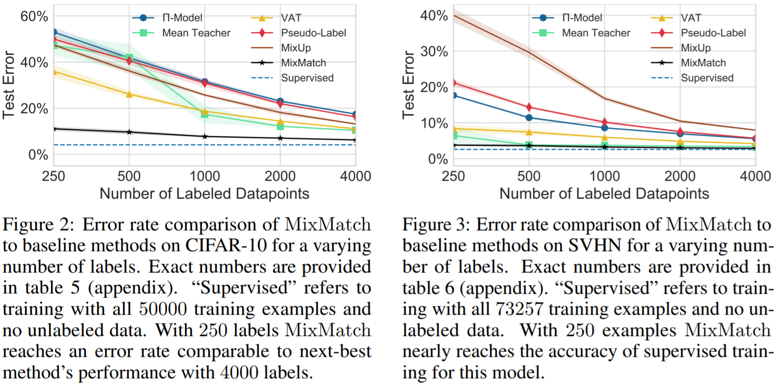 SSL Results on CIFAR-10 and SVHN
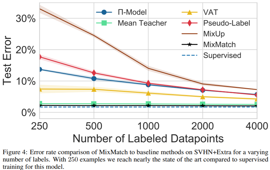 SSL Results on SVHN+Extra
Ablation Study
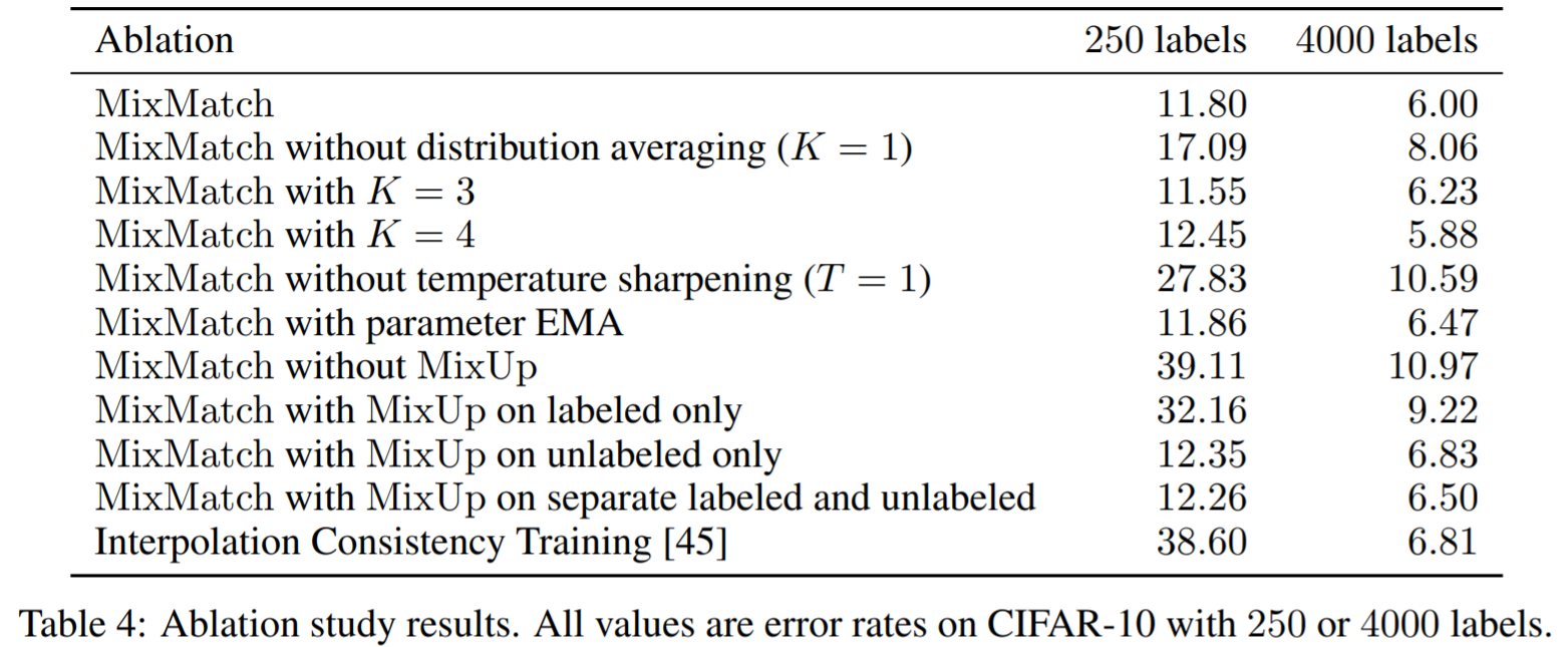 Ablation Study Results on CIFAR-10
여기까지 Semi-Supervised Learning에 대한 모델 MixMatch 에 대한 소개였습니다.!
2019년에 나온 후 ReMixMatch와 FixMatch와 같은 MixMatch에 대한 후속 연구들이 생겨났습니다.
이에 대한 소개는 다음에..! ☆