Relevance Vector Machine

Posted Feb 19, 2021 Updated Feb 11, 2024

By 12 min read

먼저, 이 글은 PRML (CH7) 공부를 바탕으로 작성된 글입니다. 따라서, 간혹 틀리다거나 더 좋은 해석이 있다면 편하게 댓글 부탁드립니다!

Relevance Vector Machine

Summary!
- RVM은 Bayesian SVM입니다!
- 특징: evidence approximation 과정에서 SVM보다 더 sparse해진다는 특징이 있습니다.
- 장점: 더 sparse한데도 성능은 꽤 좋습니다. hyper-parameter tuning은 자동적으로 결정될 수 있습니다.
- 단점: training 자체는 SVM보다 느립니다.
기존 SVM의 단점은 다음과 같습니다.
- 결과가 deterministic합니다.
- binary classification만 잘하며 multi-class classification은 잘 못합니다.
- hyper-parameter tuning은 validation을 해야 하므로 오래 걸릴 수 있습니다.
- kernel function은 positive definite이어야 하고 training data points를 중심으로 표현되어야 합니다.

1. Regression using RVM

RVM은 Bayesian SVM이므로 Bayesian Approach로 SVM을 구하고자 합니다. RVM은 GP의 한 케이스입니다. GP처럼 posterior를 구하고, hyper-parameter를 learning하고 구하면서 모델을 추정합니다.

posterior 구하기
RVM이 상정하는 모델과 분포는 다음과 같이 표현할 수 있습니다. 여기서, kernel function은 제약이 없고 어떤 basis function도 사용가능한 것이 RVM의 장점입니다. 기존의 SVM은 positive definite인 kernel function만 사용가능했습니다.
\[\begin{aligned} y(\mathbf{x})&=\sum_n^N w_n k(\mathbf{x},\mathbf{x}_n)+b \\ p(t|\mathbf{x},\mathbf{w},\beta)&=\mathcal{N}(t|y(\mathbf{x}),\beta^{-1}) \end{aligned}\]
따라서 likelihood는 다음과 같이 나타낼 수 있습니다.
\[p(\mathbf{t}|X,\mathbf{w},\beta)=\prod p(t_n|x_n,\mathbf{w},\beta^{-1})=\mathcal{N}(\mathbf{t}|\Phi\mathbf{w},\beta^{-1}I)\]
그리고 weight에 대한 prior는 다음과 같이 표현합니다.
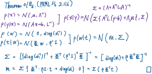
\[\begin{aligned} p(\mathbf{w}|\boldsymbol{\alpha})=\prod\mathcal{N}(w_i|\mathbf{0},\alpha_i^{-1})&=\mathcal{N}(\mathbf{w}|\mathbf{0},\textrm{diag}(\alpha_i^{-1}))=\mathcal{N}(\mathbf{w}|\mathbf{0},A^{-1}) \\ A&=\textrm{diag}(\alpha_i) \end{aligned}\]
이제, likellihood와 prior를 이용해 posterior를 구할 수 있습니다. posterior는 다음과 같이 구해지며, 증명은 아래에 있습니다.
\[\begin{aligned} p(\mathbf{w}|\mathbf{t},X,\boldsymbol{\alpha},\beta)&=\mathcal{N}(\mathbf{w}|\mathbf{m},\Sigma) \\ \mathbf{m}&=\beta\Sigma\Phi^\text{T}\mathbf{t} \\ \Sigma&=(A+\beta\Phi^\text{T}\Phi)^{-1} \end{aligned}\]
증명
1 2 ![/assets/img/posts/2021-02-18-Relevance-Vector-Machine/img1.png](/assets/img/posts/2021-02-18-Relevance-Vector-Machine/img1.png) </div>
</details>
evidence approximation을 이용해 hyper-parameter 구하기
GP에서도, Bayesian Linear Regression에서도, evidence, 즉 marginal likelihood를 maximize하여 hyper-parameter를 구할 수 있었습니다. 따라서, 기존에 하던 것처럼 marginal likelihood를 구하여 maximize하는 hyper-parameter 값을 구하면 됩니다.
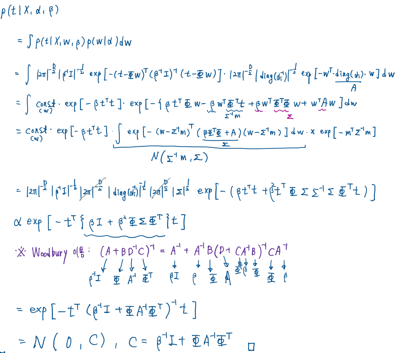
1. marginal likelihood는 Gaussian distribution의 convolution 형태이므로 Gaussian distribution으로 나타낼 수 있습니다. 분포는 다음과 같으며 증명은 아래를 참고하시면 됩니다.
  \[\begin{aligned} p(\mathbf{t}|X,\boldsymbol{\alpha},\beta)&=\int p(\mathbf{t}|X,\mathbf{w},\beta)p(\mathbf{w}|\boldsymbol{\alpha})d\mathbf{w} \\ &=\mathcal{N}(\mathbf{t}|\mathbf{0},C) \end{aligned}\] \[C=\beta^{-1}I+\Phi A^{-1}\Phi\]
  증명
  1 2 ![/assets/img/posts/2021-02-18-Relevance-Vector-Machine/img3.png](/assets/img/posts/2021-02-18-Relevance-Vector-Machine/img3.png) </div>
  </details>
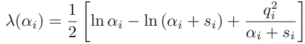
2. 이제 (log) marginal likelihood를 maximize합니다. $\begin{aligned} \ln p(\mathbf{t}|X,\boldsymbol{\alpha},\beta)&=-\frac{1}{2}\left[N\ln(2\pi)+\ln|C|+\mathbf{t}^\textrm{T}C^{-1}\mathbf{t}\right] \\ \nabla \ln p(\mathbf{t}|X,\boldsymbol{\alpha},\beta)&=-\frac{1}{2}\left[Tr[C^{-1}\frac{\partial C}{\partial \alpha_i}]+\mathbf{t}^\textrm{T}C^{-1}\frac{\partial C}{\partial \alpha_i}C^{-1}\mathbf{t}\right]=0 \end{aligned}$
  위를 풀면 다음과 같은 newer hyper-parameter를 구할 수 있습니다.
  \[\alpha_i^{new}=\frac{\gamma_i}{m_i^2},\text{ }(\beta^{new})^{-1}=\frac{\|\mathbf{t}-\Phi\mathbf{w}\|^2}{N-\sum_i\gamma_i} \\ \gamma_i=1-\alpha_i\Sigma_{ii}, m_i=[\mathbf{m}]_i, \Sigma_{ii}=[\Sigma]_{ii}\]
optimal $\alpha, \beta$ 구하는 과정 (evidence 근사 이용)
1. $\alpha, \beta$ 초깃값
  1. (posterior) mean, cov 평가
  2. hyper-parameter 재추정
  3. 수렴까지 2-3. 반복
relevance vector와 sparse 의미
relevance vector는 support vector처럼, 어떤 과정을 통해서 남은 벡터만을 이용해 모델에 학습시킨 데이터를 의미합니다. 위에서 구한 $\alpha_i$에 대해서 $\alpha_i \longrightarrow \infty$ 이면, $w_i|\alpha_i$ 의 mean과 variance가 0에 가까워지고, 실제 모델에서 $\sum w_i\phi(\mathbf{x_i})$를 계산할 때 $\phi(\mathbf{x_i})$ 값에 관계없이 0이 되므로 $\phi(\mathbf{x_i})$ 벡터가 아무 역할을 못하게 됩니다. 따라서 이러한 벡터는 제거하고, 0이 되지 않는 $w_i$에 해당하는 $\mathbf{x_i}$를 relevance vector라고 합니다. relevance 라고 하는 이유는 이러한 과정이 marginal likelihood를 maximize하는 ARD(Automatic Relevance Determination)를 통해 나오기 때문인 것 같습니다.(저의 추정)
여기서 의미하는 sparse는 위에서 relevance vector만 남고 나머지는 모델에서 제거되므로, 고려하는 데이터가 적다는 의미에서 sparse라고 합니다. 모델 자체가 적은 데이터 수로 학습이 되므로 이를 sparse model이라고 합니다. SVM에 비해 얼마나 sparse하냐면, 아래와 같습니다.
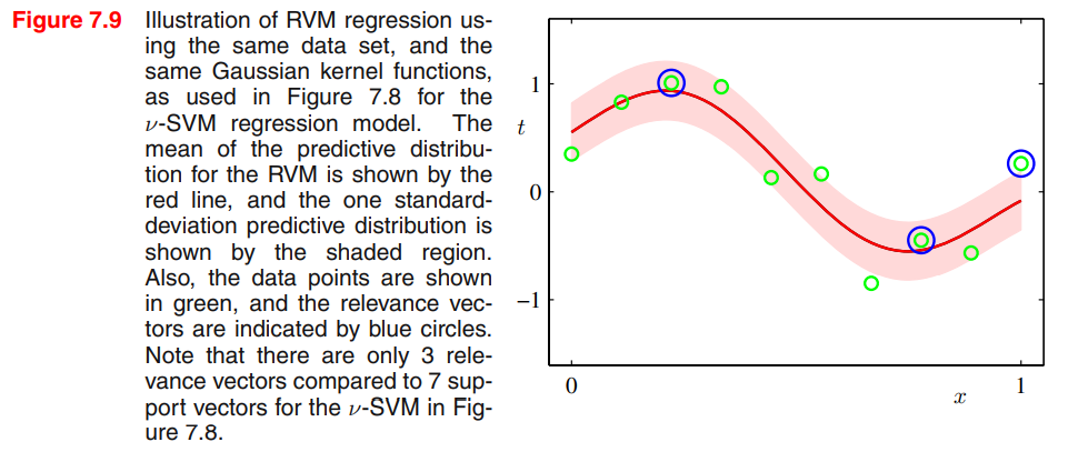source: PRML book
predictive distribution
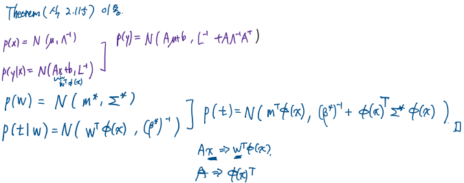
모델을 추정했으니 이번엔 예측을 합니다. 이 또한 앞의 Bayesian approach를 이용한 모델들에서 많이 다뤘습니다. 새로운 input $\mathbf{x}^*$에 대한 예측값을 $t^*$라고 하면, 식은 다음과 같고, 이에 대한 증명은 아래와 같습니다.
\[\begin{aligned} p(t^*|\mathbf{x}^*,X,\mathbf{t},\boldsymbol{\alpha}^*,\beta^*)&=\int p(t^*|\mathbf{x}^*,\mathbf{w},\beta^*)p(\mathbf{w}|X,t^*,\alpha^*,\beta^*)d\mathbf{w} \\ &=\mathcal{N}(\mathbf{t}|(\mathbf{m}^*)^\textrm{T}\phi(\mathbf{x}^*),\sigma^2(\mathbf{x}^*)) \\ \sigma^2(\mathbf{x}^*)&=(\beta^*)^{-1}+\phi(\mathbf{x}^*)^\textrm{T}\Sigma^*\phi(\mathbf{x}^*) \end{aligned}\]
증명
1 2 ![/assets/img/posts/2021-02-18-Relevance-Vector-Machine/img7.png](/assets/img/posts/2021-02-18-Relevance-Vector-Machine/img7.png) </div>
</details>
기타 논점
- localized basis function의 경우 basis function이 없는 input space의 region에서 예측분산이 작아진다. 이런 경우 RVM은 데이터 도메인 밖에서 extrapolate할수록 예측에 확신을 준다. → 멀리 있는 데이터를 relevance로 선택하게 된다?! -> degenerate of covariance function과의 연관성이 무엇인지 (?)
- RVM의 단점은 training time이 길다는 것입니다. 하지만 SVM이 hyper-parameter tuning을 위해 validation을 하고, RVM이 더 sparse하므로(모델에서 계산되는 데이터가 적으므로) 그렇게 느리지 않을 수 있습니다.

2. Analysis of Sparsity

RVM의 Sparsity(희박도)에 대한 통찰을 이 챕터에서 설명합니다. RVM의 sparsity가 어디서 어떻게 결정되는지를 간단한 예시 및 수학을 이용해 설명합니다.

예시: 그림을 이용한 직관적 설명
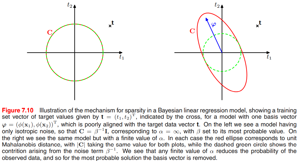
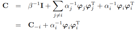
데이터가 2개인 경우, marginal likelihood와 그에 대한 covariance matrix는 다음과 같습니다.
\[p(\mathbf{t}|\alpha,\beta)=\mathcal{N}(\mathbf{t}|\mathbf{0},C) \\ C=\beta^{-1}I+\alpha^{-1}\varphi\varphi^\textrm{T}\]
- $\varphi$와 $\mathbf{t}$의 방향이 잘 align하면, 이를 relevance vector로 고려하여 모델에 포함시킵니다.
- $\varphi$와 $\mathbf{t}$의 방향이 잘 align하지 않으면,
  - $\alpha \rightarrow \infty$가 되어 해당 항이 0이 되고, 공분산에 대한 $\varphi$의 영향이 없어 모델로부터 제거됩니다.
  - $\alpha <\infty$이면(오른쪽 그림) 해당 항에 값이 주어지고 공분산이 커져(퍼져) 데이터에는 낮은 확률이 부여되어, $\mathbf{t}$에서의 밀도(확률)값이 낮아집니다. 이는 분포가 퍼지고(데이터로부터 멀어짐) → 따라서 이 경우 align하는지 안 하는지에 따라 뺄 수 있습니다. 여기서는 align하지 않은 경우이므로 데이터를 뺍니다.
source: PRML book
수학적 설명과 Sparsity와 Quality에 대한 정의
we make explicit all of the dependence of the marginal likelihood on a particular αi and then determine its stationary points explicitly
1. posterior의 covariance matrix에서 $\alpha_i$의 기여분을 따로 빼냅니다.
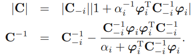
2. log likelihood는 다음과 같이 구할 수 있고,
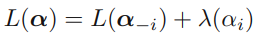
3. $\alpha_i$에 대한 dependence를 포함하는 function은 아래와 같이 계산됩니다.
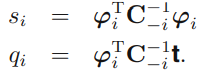
  - $s_i$ (sparsity of $\varphi_i$) : basis function이 모델의 다른 basis vector와 overlap되는 정도를 의미합니다.
  - $q_i$ (quality of $\varphi_i$) : $\mathbf{t}$와 $\mathbf{y}_{-i}$ 간 error와 basis vector $\varphi_i$가 align된 정도를 의미합니다.
Sparsity와 Quality의 상대적인 크기
1. Stationary points of the marginal likelihood with respect to $\alpha_i$
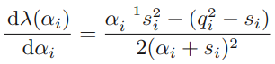
  위 식이 0이 될 때는,
  1. $\alpha_i \ge 0$일 때,
    1. $q_i^2 < s_i$일 때 : $\alpha_i \rightarrow \infty$ 가 됩니다.
    2. $q_i^2 > s_i$일 때 :
  ⇒ 따라서, 이의 상대적 크기가 basis vector가 모델에서 제거되는지 아닌지 결정하게 됩니다.
  → 이는 $\alpha_i$에 대해 closed form 형태의 해가 나타나게 됩니다.
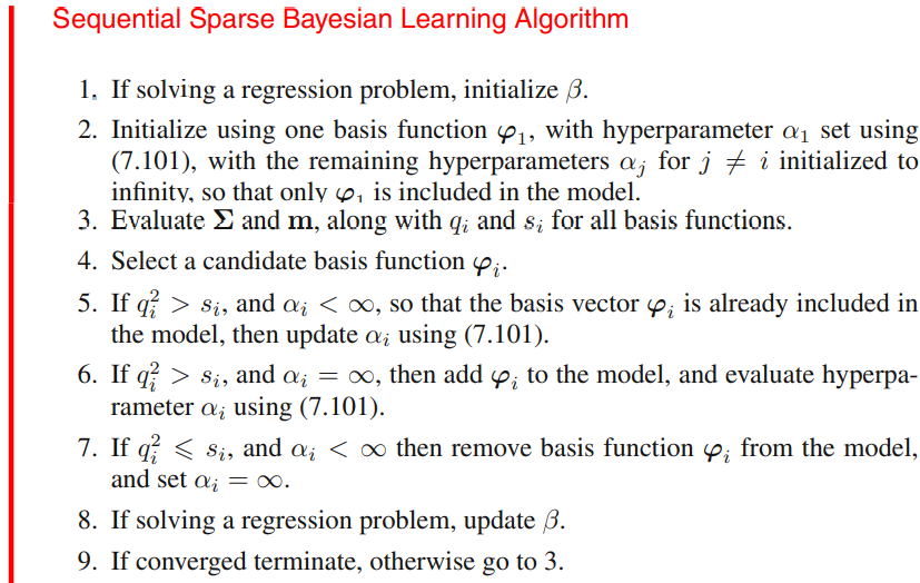
Sequential Sparse Bayesian Learning Algorithm
basis vector가 모델이 포함되는지 아닌지 반복해서 확인하는 알고리즘 입니다.
source: PRML book
efficient implementation
아래처럼 $Q$와 $S$에 대해 미리 계산하면 효율적으로 RVM을 구현할 수 있습니다.
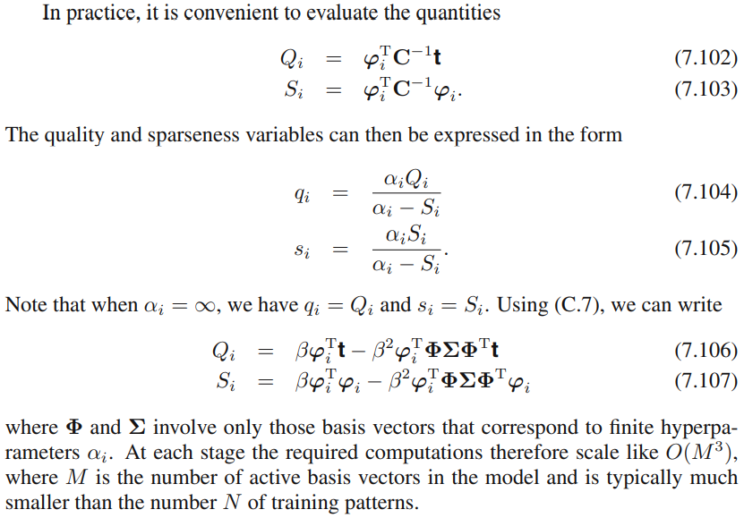source: PRML book

3. RVM for Classification

RVM을 이용해 Classification을 풀어봅시다. 이 또한 GP Classifier와 유사합니다. 다만 posterior를 근사하기 위해선 Gaussian Approximation이 필요합니다.

posterior 구하기

Classification에서 모델은 다음과 같습니다.

\[y(\mathbf{x},\mathbf{w})=\sigma(\mathbf{w}^\textrm{T}\phi(\mathbf{x}))\]

prior는 위의 regression task와 같이 다음과 같이 정의합니다.

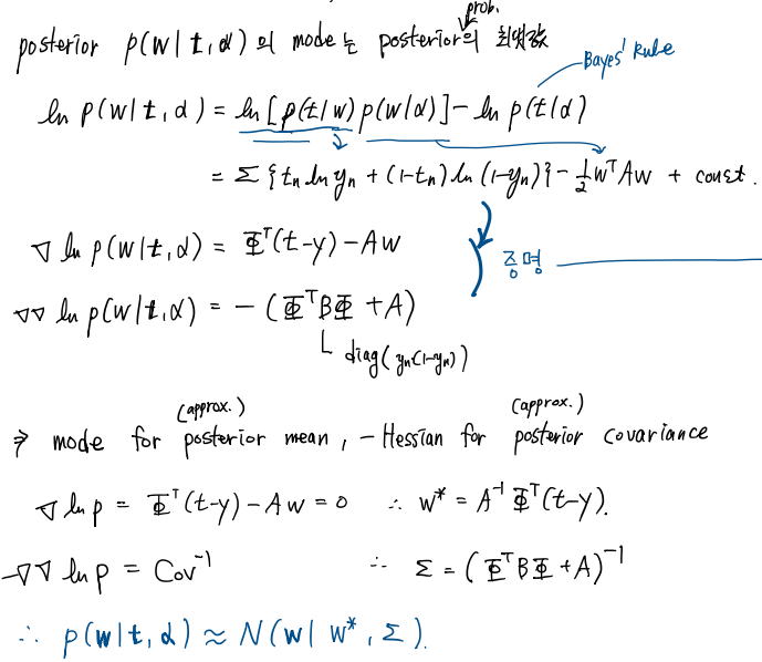
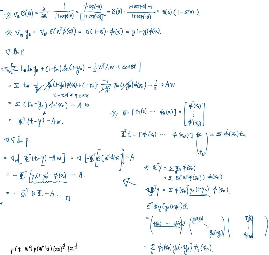
\[p(\mathbf{w}|\alpha)=\prod\mathcal{N}(w_i|0,\alpha_i^{-1})=\mathcal{N}(\mathbf{w}|\mathbf{0},\textrm{diag}(\alpha_i^{-1}))\]

Classification task에서 GP는 Gaussian approximation이 필요했습니다. 여기서는 Laplace Approximation을 이용하겠습니다. Laplace Approximation은 posterior의 mode를 가우시안의 mean, negative Hessian matrix를 covariance matrix로 근사하는 방법입니다. 이를 이용하면 posterior는 다음과 같이 구할 수 있습니다.

\[p(\mathbf{w}|\mathbf{t}|\boldsymbol{\alpha})\approx\mathcal{N}(\mathbf{w}|\mathbf{w}^*,\Sigma) \\ \mathbf{w}^*=A^{-1}\Phi^\textrm{T}(\mathbf{t}-\mathbf{y})\\ \Sigma=(\Phi^\textrm{T}B\Phi+A)^{-1}\]

gradient, Hessian 증명

     ![/assets/img/posts/2021-02-18-Relevance-Vector-Machine/img21.png](/assets/img/posts/2021-02-18-Relevance-Vector-Machine/img21.png)
     ![/assets/img/posts/2021-02-18-Relevance-Vector-Machine/img22.png](/assets/img/posts/2021-02-18-Relevance-Vector-Machine/img22.png)
 </div>

</details>

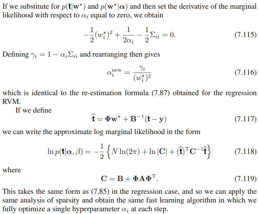
learning hyper-parameter using marginal likelihood
다음의 marginal likelihood를 maximize함으로써 hyper-parameter를 구합니다.
\[\begin{aligned} p(\mathbf{t}|\boldsymbol{\alpha})&=\int p(\mathbf{t}|\mathbf{w})p(\mathbf{w}|\boldsymbol{\alpha})d\mathbf{w} \\ &\simeq p(\mathbf{t}|\mathbf{w}^*)p(\mathbf{w}^*|\alpha)\frac{(2\pi)^{M/2}}{|\Sigma|^{1/2}} \end{aligned}\] \[\alpha_i^{new}=\frac{\gamma_i}{m_i^2}, \quad \gamma_i=1-\alpha_i\Sigma_{ii}\]
re-estimated hyper-parameter 증명
1 2 3 (아직 미완성) 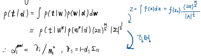![/assets/img/posts/2021-02-18-Relevance-Vector-Machine/img23.png](/assets/img/posts/2021-02-18-Relevance-Vector-Machine/img23.png) </div>
</details>
$\alpha$ 구하는 과정
1. $\alpha$ 초기화
2. initial $\alpha$에 대한 posterior의 Gaussian approximation (marginal likelihood)
3. \[\alpha=\arg\max marginal\text{ }likelihood\]
4. 수렴까지 2-3. 반복
기타 논점
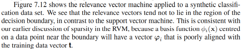
- Analysis of Sparsity: classfication case
  source: PRML book
- relevance vector가 decision boundary 쪽에 없다는 것은 $\phi_i(\mathbf{x})$와 $\mathbf{t}$가 잘 align해서 0이 안된 경우이고, 잘 align하지 않으면 0이 되므로 sparse해진다. (잘 align하지 않은 애들은 decision boundary 근처에 있는 애들)
  source: PRML book
  source: PRML book